Abstract

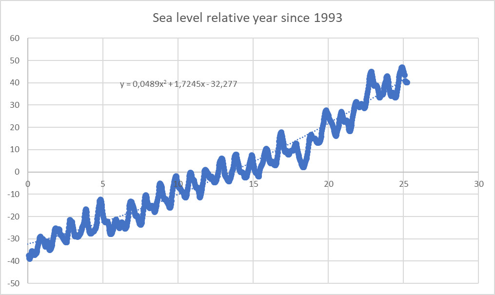
The element of random walk in natural processes can be discussed if we consider the figures as a function of time and as control- or nullhypothesis for the deterministic model of sea level change. Generally sea level change are thought to be determined by land ice melting and thermal expansion of the oceans. In this article I will not discuss that side of the case but merely what the numbers can tell without any implication of cause and effect. Can the time series be reproduced as a random walk by dividing the series in two parts: one which contains the uptics and one contains the downticks. Are the uptics very different from the downtics although the series over time shows a generally increasing sea level and even an accelerated pace? In the random statistic model called Kolmogorov-Smirnoff the degree of randomness can be dertermined independent of time and amount of points in each series. Additionaly also Bernoulli test can also be used as a test of whether or not an uptick and a downtick have a 50% chance to occur in the time series.

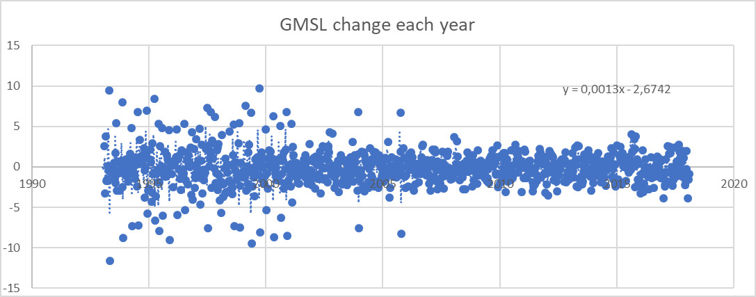
In this informal article I can show some evidence for a random walk in the sea level change 1993-2018 and also a Bernoulli test pointing in the same direction.

Whether these processes are only random walk we can not decide but a validation of the increase in time of a measured natural phenomenon as a decisive proof of significance can be considered an oversimplification or perhaps too naive.

K-S test on GMSL data from NASA

KS Test: Results

Kolmogorov-Smirnov Comparison of Two Data Sets by http://www.physics.csbsju.edu/cgi-bin/stats/KS-test.n.plot

The results of a Kolmogorov-Smirnov test performed at 06:03 on 21-MAY-2018

The maximum difference between the cumulative distributions, D, is: 0.0477 with a corresponding P of: 0.662

Data Set 1:

466 data points were entered
Mean = 1.517
95% confidence interval for actual Mean: 1.372 thru 1.661
Standard Deviation = 1.59
High = 9.89 Low = 0.01
Third Quartile = 1.99 First Quartile = 0.510
Median = 1.070
Average Absolute Deviation from Median = 1.01

John Tukey defined data points as outliers if they are 1.5*IQR above the third quartile or below the first quartile. Following Tukey, the following data points are outliers: 9.89 9.61 8.62 8.19 7.72 7.48 7.16 6.98 6.97 6.95 6.92 6.86 6.85 6.43 6.40 5.62 5.56 5.53 5.50 5.46 5.37 5.20 5.00 5.00 4.91 4.82 4.77 4.71 4.58 4.48 4.47 4.30

KS says it’s unlikely this data is normally distributed: P= 0.00 where the normal distribution has mean= 3.073 and sdev= 1.872

KS says it’s unlikely this data is log normally distributed: P= 0.00 where the log normal distribution has geometric mean= 0.6007 and multiplicative sdev= 4.058

Items in Data Set 1:

1.000E-02 1.000E-02 1.000E-02 1.000E-02 2.000E-02 2.000E-02 2.000E-02 3.000E-02 3.000E-02 3.000E-02 4.000E-02 4.000E-02 4.000E-02 4.000E-02 4.000E-02 4.000E-02 5.000E-02 5.000E-02 6.000E-02 6.000E-02 7.000E-02 7.000E-02 7.000E-02 7.000E-02 8.000E-02 8.000E-02 8.000E-02 9.000E-02 9.000E-02 9.000E-02 0.100 0.100 0.120 0.120 0.120 0.120 0.120 0.130 0.140 0.140 0.150 0.150 0.150 0.150 0.160 0.160 0.160 0.170 0.170 0.180 0.180 0.180 0.180 0.190 0.190 0.200 0.210 0.210 0.220 0.220 0.220 0.220 0.220 0.230 0.250 0.250 0.250 0.250 0.260 0.270 0.270 0.280 0.280 0.280 0.280 0.280 0.290 0.290 0.290 0.300 0.300 0.300 0.300 0.310 0.320 0.330 0.340 0.360 0.360 0.360 0.370 0.370 0.370 0.380 0.380 0.380 0.390 0.390 0.390 0.390 0.400 0.400 0.400 0.410 0.410 0.420 0.420 0.430 0.440 0.450 0.450 0.450 0.450 0.450 0.490 0.510 0.510 0.520 0.520 0.520 0.530 0.540 0.540 0.540 0.540 0.550 0.570 0.570 0.570 0.590 0.590 0.610 0.610 0.610 0.610 0.620 0.620 0.620 0.630 0.630 0.630 0.630 0.640 0.650 0.650 0.650 0.660 0.660 0.670 0.670 0.690 0.690 0.690 0.690 0.690 0.690 0.700 0.700 0.710 0.720 0.730 0.730 0.740 0.750 0.750 0.760 0.770 0.770 0.780 0.780 0.780 0.790 0.790 0.790 0.790 0.790 0.800 0.800 0.810 0.820 0.820 0.830 0.830 0.840 0.850 0.860 0.860 0.860 0.860 0.860 0.870 0.870 0.870 0.870 0.870 0.870 0.880 0.890 0.910 0.910 0.920 0.920 0.920 0.930 0.930 0.930 0.930 0.940 0.940 0.940 0.950 0.950 0.950 0.950 0.960 0.960 0.970 0.970 0.980 0.980 0.980 0.990 1.00 1.01 1.01 1.02 1.02 1.03 1.04 1.05 1.06 1.07 1.07 1.07 1.08 1.08 1.09 1.09 1.10 1.10 1.11 1.11 1.11 1.12 1.12 1.12 1.13 1.13 1.13 1.13 1.13 1.13 1.14 1.14 1.14 1.15 1.15 1.15 1.15 1.15 1.16 1.16 1.17 1.17 1.18 1.18 1.18 1.21 1.21 1.23 1.26 1.26 1.28 1.28 1.29 1.30 1.30 1.33 1.34 1.34 1.34 1.35 1.36 1.36 1.36 1.38 1.40 1.41 1.41 1.41 1.41 1.41 1.42 1.44 1.44 1.44 1.45 1.45 1.45 1.47 1.48 1.49 1.52 1.52 1.53 1.54 1.57 1.57 1.58 1.59 1.60 1.60 1.60 1.61 1.61 1.62 1.62 1.64 1.65 1.65 1.66 1.66 1.66 1.67 1.70 1.71 1.73 1.74 1.76 1.80 1.83 1.85 1.88 1.88 1.89 1.90 1.90 1.91 1.92 1.93 1.93 1.94 1.94 1.97 1.97 1.97 1.98 1.98 1.99 1.99 1.99 2.00 2.00 2.01 2.01 2.02 2.02 2.03 2.03 2.03 2.06 2.06 2.07 2.07 2.08 2.10 2.12 2.12 2.13 2.16 2.21 2.22 2.22 2.22 2.23 2.25 2.25 2.25 2.25 2.32 2.32 2.33 2.33 2.33 2.37 2.37 2.39 2.42 2.46 2.47 2.47 2.48 2.54 2.56 2.56 2.56 2.59 2.62 2.62 2.62 2.67 2.71 2.71 2.73 2.73 2.74 2.74 2.75 2.80 2.82 2.83 2.87 2.90 2.91 2.92 2.95 2.96 2.97 2.99 3.07 3.10 3.13 3.22 3.23 3.37 3.47 3.53 3.61 3.64 3.89 3.91 3.91 4.15 4.20 4.30 4.47 4.48 4.58 4.71 4.77 4.82 4.91 5.00 5.00 5.20 5.37 5.46 5.50 5.53 5.56 5.62 6.40 6.43 6.85 6.86 6.92 6.95 6.97 6.98 7.16 7.48 7.72 8.19 8.62 9.61 9.89

Data Set 2:

455 data points were entered

Mean = 1.557

95% confidence interval for actual Mean: 1.407 thru 1.708

Standard Deviation = 1.63

High = 11.5 Low = 0.00

Third Quartile = 1.95 First Quartile = 0.550

Median = 1.110

Average Absolute Deviation from Median = 1.00

John Tukey defined data points as outliers if they are 1.5*IQR above the third quartile or below the first quartile. Following Tukey, the following data points are outliers: 11.5 9.27 8.85 8.58 8.53 8.33 8.08 7.89 7.76 7.41 7.40 7.31 7.16 7.11 7.02 6.49 6.11 5.87 5.77 5.57 5.48 5.20 5.15 4.46 4.26 4.14

KS says it’s unlikely this data is normally distributed: P= 0.00 where the normal distribution has mean= 3.310 and sdev= 2.058

Items in Data Set 2:

0.00 1.000E-02 1.000E-02 1.000E-02 2.000E-02 2.000E-02 3.000E-02 3.000E-02 3.000E-02 5.000E-02 6.000E-02 7.000E-02 7.000E-02 7.000E-02 7.000E-02 9.000E-02 9.000E-02 0.100 0.100 0.100 0.110 0.110 0.120 0.130 0.130 0.130 0.140 0.140 0.140 0.140 0.150 0.150 0.150 0.160 0.160 0.160 0.160 0.160 0.160 0.180 0.180 0.190 0.190 0.200 0.200 0.200 0.210 0.210 0.220 0.230 0.230 0.240 0.240 0.240 0.240 0.250 0.250 0.250 0.260 0.260 0.260 0.270 0.280 0.280 0.280 0.290 0.290 0.290 0.300 0.300 0.310 0.310 0.320 0.330 0.340 0.350 0.360 0.360 0.360 0.380 0.380 0.380 0.380 0.380 0.390 0.390 0.400 0.410 0.430 0.440 0.440 0.450 0.460 0.470 0.470 0.480 0.490 0.490 0.490 0.500 0.500 0.500 0.510 0.520 0.520 0.520 0.530 0.530 0.550 0.550 0.550 0.550 0.550 0.550 0.560 0.570 0.580 0.590 0.590 0.590 0.600 0.600 0.600 0.610 0.610 0.620 0.620 0.630 0.630 0.640 0.640 0.640 0.650 0.650 0.660 0.670 0.670 0.670 0.690 0.690 0.700 0.700 0.700 0.710 0.710 0.710 0.720 0.720 0.730 0.730 0.730 0.730 0.740 0.750 0.760 0.760 0.760 0.770 0.770 0.780 0.780 0.780 0.780 0.780 0.790 0.800 0.810 0.820 0.830 0.830 0.840 0.840 0.850 0.850 0.850 0.850 0.860 0.870 0.870 0.870 0.880 0.890 0.900 0.900 0.910 0.910 0.920 0.920 0.920 0.920 0.940 0.950 0.950 0.950 0.950 0.960 0.960 0.960 0.960 0.960 0.970 0.970 0.990 0.990 1.01 1.01 1.01 1.01 1.03 1.03 1.03 1.03 1.04 1.06 1.06 1.06 1.06 1.07 1.08 1.09 1.09 1.10 1.10 1.10 1.11 1.11 1.11 1.11 1.12 1.12 1.14 1.15 1.15 1.15 1.16 1.16 1.16 1.18 1.18 1.20 1.20 1.20 1.21 1.22 1.22 1.22 1.23 1.23 1.23 1.24 1.24 1.24 1.24 1.25 1.25 1.28 1.29 1.31 1.33 1.33 1.34 1.35 1.36 1.36 1.38 1.38 1.39 1.40 1.41 1.41 1.42 1.42 1.42 1.42 1.44 1.45 1.45 1.46 1.46 1.46 1.48 1.49 1.49 1.49 1.49 1.50 1.50 1.51 1.51 1.52 1.52 1.53 1.55 1.55 1.55 1.56 1.57 1.60 1.60 1.62 1.62 1.62 1.63 1.64 1.65 1.65 1.66 1.66 1.68 1.70 1.70 1.70 1.73 1.73 1.73 1.74 1.75 1.76 1.76 1.76 1.77 1.79 1.79 1.79 1.82 1.83 1.84 1.86 1.86 1.87 1.87 1.87 1.88 1.91 1.91 1.91 1.91 1.92 1.93 1.94 1.94 1.95 1.95 1.95 1.95 1.96 1.96 1.97 1.97 2.02 2.03 2.04 2.11 2.15 2.17 2.18 2.18 2.21 2.22 2.22 2.22 2.22 2.23 2.23 2.25 2.25 2.28 2.29 2.30 2.31 2.31 2.35 2.39 2.40 2.40 2.40 2.43 2.43 2.43 2.45 2.45 2.47 2.48 2.48 2.50 2.50 2.54 2.55 2.58 2.60 2.61 2.63 2.65 2.66 2.72 2.72 2.73 2.74 2.77 2.78 2.78 2.80 2.81 2.84 2.87 2.89 2.89 2.93 2.94 2.95 3.02 3.03 3.07 3.07 3.10 3.10 3.13 3.15 3.31 3.32 3.43 3.45 3.49 3.63 3.63 3.70 3.74 3.89 3.99 4.14 4.26 4.46 5.15 5.20 5.48 5.57 5.77 5.87 6.11 6.49 7.02 7.11 7.16 7.31 7.40 7.41 7.76 7.89 8.08 8.33 8.53 8.58 8.85 9.27 11.5

Data Reference: 4F37

Referanser

https://en.wikipedia.org/wiki/Kolmogorov–Smirnov_test